Two Boundaries for Simulated People: Documented Individuals and Unsurveyed Populations
Introduction
A prior study of one survey-grounded persona system reached two negative-sounding conclusions and named two escape routes it did not test (Grey 2026). At the individual level, persona traits sampled from a person’s demographics cannot predict that person better than the demographics alone, and empirically they predict worse, because the language model obeys the invented label and discards its own priors. At the population level, grounded personas beat naive repeated prompting decisively but merely tie a direct question, a verbalized-sampling prompt, a single calibrated label, or a lookup table built from the generator’s own training data. The escape routes were stated as structural arguments rather than measurements. First, the individual-level limit is a theorem about invented people: for a documented person whose attributes are measured rather than sampled, its premise fails and the argument should invert. Second, the population-level ties were all measured on coarse, heavily surveyed cells; where no survey has published a number, a lookup has no row and a language model has nothing to recall, while a generative joint model can still answer.
This paper measures both.
Study 3 (§4) asks how much you must know about someone. We hold the pipeline fixed and vary only the provenance of what a persona knows about itself: nothing beyond demographics, traits sampled from those demographics, or attributes the person actually reported, for from 1 to 16. The unit is a real ANES 2020 respondent, which is a documented individual in the only sense that admits ground truth: a real person with a large set of measured attributes and held-out outcomes measured on the same instrument. Four questions follow. Where is the crossing point at which disclosure beats the demographic baseline? Does simulating a person in character ever beat simply asking about them, given the same facts? Does a zero-shot language model beat a supervised model fitted on thousands of labelled respondents with the same attributes? And does wrong but plausible detail hurt — the safety question that decides whether provenance is a feature or a slogan.
Study 4 (§5) asks where asking stops working. We deepen the audience specification from one fixed demographic attribute to five and watch every arm degrade. Two things make the deep regime different in kind rather than degree. The lookup baseline’s degradation is visible: it must back off to coarser conditionals and can report that it did. The direct-readout arm’s degradation is invisible: it answers a five-way question as fluently as a one-way question. And the ground truth itself degrades, so the study is only interpretable with a measured floor beneath it — which we estimate per cell and draw beneath every comparison.
Both escapes turn out to be real and narrower than advertised. The individual-level inversion is large — about a quarter of the accuracy scale, on all three models, from a single disclosed attribute — and it is entirely explained by the model complying with what it was told, including when what it was told belongs to somebody else. The deep-population escape mostly is not there: the direct arm degrades fastest but stays ahead, prompting for a spread degrades least, and the free arms turn out not to degrade with depth at all once cell mass is controlled, because their apparent decline was the reference survey thinning rather than the generator failing.
Our contributions:
A controlled measurement of persona provenance: the same pipeline, elicitor and respondents with only the origin of the persona’s attributes varying, giving the first dose-response curve for how much you must know about a person before simulating them beats describing them demographically, together with the two controls — a matched-stranger placebo and a supervised model on the same attributes — that decide whether a gain is information or compliance (§4).
An obedience measurement that separates the two: language models track a disclosed attribute more tightly than the attribute tracks the outcome, and track a stranger’s attribute nearly as tightly, which makes provenance an external enforcement problem rather than something the model can be trusted to weigh (§4).
A depth curve for population readout with the reference survey’s own sampling error measured per cell and drawn beneath every comparison, and a mass control that reassigns most of the apparent depth degradation to the survey rather than to the arms (§5).
A transfer test that bounds the paper’s own headline: on the weakest-signal outcome in the same item pool the disclosure effect essentially disappears, while the placebo still hurts — exactly what a compliance mechanism predicts and an information mechanism does not (§4.5).
Two negative results that a vendor would rather not have: the structured extraction pipeline never beats pasting the source text into a prompt, and a training-support statistic that looks like a shippable confidence indicator when pooled predicts nothing within depth (§4.6, §5).
A preregistration subjected to adversarial review before any spend, with the six blocking defects it found — including a hardcoded gate and a coverage rule that made a robustness check identical to its own headline — reported rather than quietly fixed (§3.1, Appendix 10).
Related work
Individual-level persona prediction from measured data is the regime Park et al. (2024) established with two-hour interviews and Li and Conrad (2026) with behavioural traces; both report substantial gains where population-sampled traits report none (Hu and Collier 2024; Taday Morocho et al. 2026). Our Study 3 sits between those literatures by construction: it varies provenance while holding the pipeline, the elicitor and the respondent fixed, so the sampled-versus-measured contrast is a controlled comparison rather than a comparison across systems, and it adds the dose-response those studies do not report — accuracy as a function of how much is known. It also adds the two controls that decide whether the gain is information or compliance: a placebo persona carrying a demographically matched stranger’s answers, and a supervised model fitted on the same attributes.
Two literatures bracket Study 4 and we position against both. Statistical population synthesis has been generating joint microdata from marginals for two decades, most recently with deep generative models (Borysov et al. 2019), and its central difficulty — rare feature combinations that the training sample never observed — is exactly the regime we set out to reach. Our finding that we could not reach it by crossing coarse demographics is a statement about the ANES-sized reference survey, not about that literature’s problem, and we say which. On the estimation side, multilevel regression with poststratification is the canonical method for small electoral subgroups (Ghitza and Gelman 2013); our lookup baseline with hierarchical backoff is a deliberately simpler member of that family, and its strength against the generative arm should be read as a lower bound on what proper partial pooling would achieve.
The diversity side of the literature bears on Study 4’s one positive result. Alignment training is known to narrow output distributions (Kirk et al. 2024; Padmakumar and He 2024), which is the mechanism behind the variance collapse that Bisbee et al. (2024) documented in synthetic samples and that Zhang et al. (2025) recover by prompting. That grounded personas hold their within-cell dispersion inside the preregistered band at every depth we test is a claim about coverage rather than accuracy, and it is the one place our measurements favour simulation.
Population-level work has concentrated on cells that surveys report. Argyle et al. (2023) established distributional fidelity on demographic subgroups; Santurkar et al. (2023) and Bisbee et al. (2024) characterised its failures; Cao et al. (2025) fine-tune toward survey distributions and Zhang et al. (2025) recover diversity by prompting. The regime where no published number exists has been argued for rather than measured. Our Study 4 measures it, and in doing so has to confront a problem the shallow regime never posed: the reference survey’s own sampling error, which we estimate with a stratified-PSU bootstrap on the ANES variance design and report as a floor beneath every comparison. Miranda and Balbi (2025) argue LLM survey predictions should be benchmarked against supervised models; we extend that standard to same-data lookups and, in the deep regime, find the benchmark harder to beat than the shallow regime suggested.
System and shared method
Both studies use the persona system, elicitor, and held-out criterion
described in Grey
(2026), unchanged. Briefly: an eight-dimensional latent factor
model is fit over a 270,479-cell American Community Survey
backbone using 4.87M sparse observations from mounted survey sources
(Cooperative Election Study, General Social Survey, CPS Voting and
Registration, Big Five inventories, Moral Foundations Questionnaire,
Pol.is aggregates, Voteview, EJScreen). A persona is one draw: a
backbone cell, a latent vector, and decoded attributes. The ANES is not
among the training sources, so it is genuinely held out. All runs here
use the calibrated artifact
fusion-v1-party-ordinal-cal3-2026-08-15 at latent
temperature 1.0 — the product default, and the policy for every run
after 2026-08-15.
Elicitation is the same single-shot in-character survey call in both studies, and every arm within a study differs only in the persona text supplied. Targets are the 2020 presidential vote and the 7-point party identification, and are never disclosed to any arm.
Preregistration and run integrity
Both studies were preregistered before any paid call: hypotheses, arms, cells or splits, metrics, decision rules and budget ceilings were written down and are reproduced in Appendix 10. Amendments made after the free stages ran and before any money was spent are listed there too, with the reason for each; nothing was amended after seeing a paid result.
Three run-integrity checks are built into both harnesses, each
installed after a specific past failure in this program: an OpenRouter
balance preflight sized from the actual work list, a per-call abort on
payment failure, and a summary that reports n_failed and
exits non-zero rather than averaging over whatever happened to
succeed.
Study 3: the disclosure curve
What plays the role of a documented individual
The claim under test concerns a specific person about whom real material exists. Testing it needs three things at once: a person with many measured attributes, a held-out outcome for that same person measured on the same instrument, and certainty that the language model is not simply recalling who they are. Public figures give the first and, with work, the second, but destroy the third.
An ANES 2020 respondent gives all three. They are a real person who
answered roughly 1,700 items; their vote and party
identification are measured alongside everything else; and no model can
have memorised respondent anes2020-03177. The design cost
is external validity — survey codes are cleaner than journalism — and
Study 3B (§4.6) is built to buy some of it
back.
The decisive property is that this holds the entire pipeline fixed while varying only provenance. The same respondents, elicitor, renderer, demographic block, temperature and targets as the prior study’s Study 1; only the origin of the persona’s self-knowledge changes.
The attribute pool
Twenty-two ANES 2020 pre-election items were verified one at a time against the official codebook — variable id, question wording, and every value label — and frozen with a first-person rendering and a third-person clause each. They span ideology, religiosity, economic policy, social policy, immigration, federal spending priorities, institutional trust, and political engagement (Appendix 11).
Nothing in the pool touches party identification or its components, presidential vote, turnout, registration, primary vote, 2016 vote, candidate thermometers or trait batteries, or “which party handles better”. Those are the targets or direct encodings of them.
One rule fixed before any outcome was inspected did real work, and it took an adversarial review to make it work correctly. An item must be answered by at least 90% of the voter population to enter the study. All twenty-two clear it — but only after a correction. “Haven’t thought much about this” had been treated as missing rather than as the disclosable fact about a person that it is, which pushed all five ANES seven-point scales below the floor, the seven-point ideology self-placement among them at 86.4%. Dropping ideology then made the study’s own without-ideology robustness check identical to the result it was checking (Appendix 10, item 1). Recoded as a named level at the scale midpoint, ideology covers 0.999, enters the ranking at rank 2, and the robustness check is a real check again (0.896 against 0.906 at ). All twenty-two items are answered completely by 5,754 of 6,222 voters (92.5%), and those complete cases are the study population, so every disclosure level is evaluated on identical respondents.
Ideology is nearly collinear with party identification, one of the two targets, so a sceptical reader is right to want it isolated. The study answers that by measurement rather than exclusion: the primary disclosure curve is P2w, which removes the three most predictive items — ideology among them.
The order in which attributes are disclosed is their fit-split predictive value, estimated on 5,354 respondents disjoint from every respondent the language models ever see.
Arms
Four hundred respondents, drawn from the complete cases with
probability proportional to survey weight, are evaluated on three models
spanning the calibration range the prior study found decisive
(deepseek-chat-v3.1, the best-calibrated baseline;
gpt-4o-mini and claude-haiku-4.5, the two
worst). Every arm shares the same demographic block and the same
elicitor at temperature 0.
| Arm | Persona content |
|---|---|
| P0 | demographics only — the prior study’s baseline |
| P1 | the prior study’s grounded arm verbatim: fusion-sampled traits, interview renderer, mode decode |
| P1-flat | the same sampled traits rendered in P2’s format, so sampled-versus-measured is not confounded with wording |
| P2() | demographics plus the respondent’s own measured attributes, |
| P2w(8) | eight attributes drawn from a pool with the three most predictive items removed |
| P3(8) | placebo: eight attributes belonging to a demographically matched different respondent |
| P4() | direct: the same facts in the third person, asked as a probability rather than acted out, |
Two arms exist only to close objections a result would otherwise invite. P2w answers “you disclosed something that is nearly the vote” with a measurement: the highest-ranked item correlates 0.782 with the vote on the fit split, so P2w removes it and its two nearest rivals — ideology and the environment-versus-business scale — and asks whether the effect survives. P3 answers “any rich detail would help” by supplying rich detail that belongs to somebody else; donors matched on a mean of 5.61 of six demographic fields, so the false attributes are demographically plausible, which is what makes the arm a placebo rather than a straw man.
Alongside every arm, and never described as a ceiling, sits a weighted logistic model fitted on the 5,354-respondent fit split with the same attributes.
Results
20,400 calls, no failures, every arm parsed for 98% of respondents. Table 1 gives every arm on every model against the demographics-only baseline, matched-sample, with paired bootstrap intervals and a three-way verdict: resolved past the non-interpretation bound, resolved but inside it, or indistinguishable from zero.
The inversion is large and it happens immediately.
One measured attribute takes balanced accuracy from 0.60–0.64 to 0.86–0.88 on all three models. The crossing point is 1. On the weak pool — the ranking with its three most predictive items removed — one attribute still gives 0.77–0.79, resolved past the bound on every model. Whatever else is true, knowing one real thing about a person is worth far more than any amount of demographic description.
Sampled traits still lose, on the same respondents, in the same run.
Arm P1 reproduces the prior study’s grounded arm and lands at 0.49–0.52, below the baseline on all three models. P1-flat, the same sampled traits rendered in the measured arm’s format, lands at 0.49–0.51, so the deficit is not a wording artefact. The contrast that matters is within one table: measured attributes , sampled attributes to , same pipeline, same people. The Proposition holds where its premise holds and inverts where it does not, and the size of the inversion is about a quarter of the accuracy scale.
Part of the reason is visible in what the generator can offer. Not
one of the issue positions carrying the individual-level signal exists
in its output schema; its issue_stances field decodes
empty. The sampled arm is not a diluted version of the measured arm — it
is a different set of fields, none of which is the one that matters.
Provenance is worth about 0.30, and the placebo says why.
The primary provenance contrast, P2(8) against the placebo P3(8) — eight fields either way, identical format, only the owner of the answers differing — is , and across the three models, every interval resolved past the bound. Against the demographics-only baseline the placebo runs to , below zero on all three with intervals excluding zero but not clearing the bound. So a persona wearing a demographically plausible stranger’s opinions is somewhat worse than one wearing no opinions at all, and dramatically worse than one wearing the subject’s own.
The mechanism is compliance, not inference.
Recomputing the prior study’s obedience statistic on these logs settles what the gain is made of. In the same respondents, the top-ranked item correlates with the vote. With the item withheld, the models’ predictions correlate to with it — their demographic prior. With it disclosed, they correlate to . The models follow a disclosed attribute more tightly than that attribute actually predicts the outcome. And in the placebo arm, where the attribute belongs to somebody else, they follow it at to : essentially the same grip on a fact that is false about this person. Obedience is not conditional on provenance, which is precisely why provenance has to be enforced outside the model.
Simulating the person is not better than asking about them.
At every disclosure level, on every model, the in-character arm and
the third-person direct arm are statistically equivalent within the
bound; eight of nine contrasts are indistinguishable from zero and the
ninth
(
on claude-haiku-4.5 at
)
does not clear it. The two arms agree on the same respondent 92–96% of
the time. Whatever the persona framing adds, it is not accuracy: the
model is performing the same inference in costume.
More disclosure stops helping the model long before it stops helping a regression.
The supervised reference improves monotonically across the weak pool,
0.822 at
to 0.894 at
.
The language models do not: gpt-4o-mini runs 0.770, 0.699,
0.718, 0.785, 0.689 across the same levels, and the other two wander
similarly. By
the fitted model leads every language model on both balanced accuracy
(0.894 versus 0.689–0.808 on the weak pool) and log loss (0.293 versus
0.316–0.320 for the best-calibrated LLM arm). A model handed one strong
fact matches a regression handed the same fact; handed sixteen, it falls
behind the regression, because it has no way to weigh them against each
other.
The comparison is not an artefact of choosing a weak learner. Fitting gradient-boosted trees, histogram gradient boosting and a random forest on the identical splits, encoding and target moves the supervised side up: on the weak pool at , gradient boosting reaches 0.905 against logistic regression’s 0.888 and the best language-model arm’s 0.808. At the ordering is the reverse and the margin is small (0.818 boosted, 0.828 logistic, 0.767–0.788 for the models). A stronger learner widens the gap exactly where the claim is made — as disclosure grows — which is what the claim predicts.
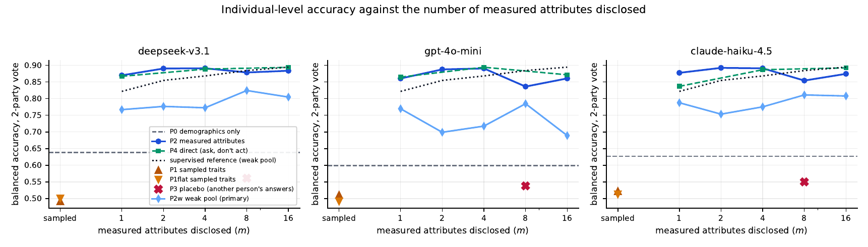
| Arm | Bal. acc. | vs P0 | 95% CI | Verdict |
|---|---|---|---|---|
| deepseek-v3.1 | ||||
| P0 demographics only | 0.638 | — | — | — |
| P1 sampled (interview) | 0.492 | -0.146 | [-0.209, -0.081] | resolved bound |
| P1-flat sampled (matched format) | 0.500 | -0.138 | [-0.203, -0.074] | , unresolved |
| P2w(1) | 0.767 | +0.128 | [+0.085, +0.173] | resolved bound |
| P2w(2) | 0.777 | +0.138 | [+0.099, +0.179] | resolved bound |
| P2w(4) | 0.772 | +0.134 | [+0.081, +0.188] | resolved bound |
| P2w(8) | 0.824 | +0.186 | [+0.133, +0.238] | resolved bound |
| P2w(16) | 0.805 | +0.166 | [+0.114, +0.220] | resolved bound |
| P2(1) | 0.870 | +0.231 | [+0.182, +0.280] | resolved bound |
| P2(2) | 0.890 | +0.252 | [+0.200, +0.304] | resolved bound |
| P2(4) | 0.891 | +0.253 | [+0.201, +0.302] | resolved bound |
| P2(8) | 0.878 | +0.240 | [+0.187, +0.293] | resolved bound |
| P2(16) | 0.883 | +0.245 | [+0.192, +0.298] | resolved bound |
| P3(8) placebo, stranger’s answers | 0.561 | -0.077 | [-0.141, -0.013] | , unresolved |
| P4(1) | 0.867 | +0.229 | [+0.178, +0.278] | resolved bound |
| P4(4) | 0.888 | +0.250 | [+0.198, +0.300] | resolved bound |
| P4(16) | 0.894 | +0.255 | [+0.205, +0.306] | resolved bound |
| gpt-4o-mini | ||||
| P0 demographics only | 0.599 | — | — | — |
| P1 sampled (interview) | 0.511 | -0.088 | [-0.144, -0.030] | , unresolved |
| P1-flat sampled (matched format) | 0.491 | -0.108 | [-0.170, -0.045] | , unresolved |
| P2w(1) | 0.770 | +0.171 | [+0.125, +0.215] | resolved bound |
| P2w(2) | 0.699 | +0.100 | [+0.057, +0.143] | , unresolved |
| P2w(4) | 0.718 | +0.118 | [+0.068, +0.168] | , unresolved |
| P2w(8) | 0.785 | +0.186 | [+0.139, +0.233] | resolved bound |
| P2w(16) | 0.689 | +0.090 | [+0.040, +0.141] | , unresolved |
| P2(1) | 0.860 | +0.261 | [+0.208, +0.314] | resolved bound |
| P2(2) | 0.888 | +0.288 | [+0.237, +0.338] | resolved bound |
| P2(4) | 0.890 | +0.291 | [+0.242, +0.340] | resolved bound |
| P2(8) | 0.836 | +0.237 | [+0.187, +0.288] | resolved bound |
| P2(16) | 0.861 | +0.261 | [+0.212, +0.312] | resolved bound |
| P3(8) placebo, stranger’s answers | 0.538 | -0.061 | [-0.119, -0.002] | , unresolved |
| P4(1) | 0.865 | +0.265 | [+0.215, +0.315] | resolved bound |
| P4(4) | 0.894 | +0.295 | [+0.246, +0.343] | resolved bound |
| P4(16) | 0.871 | +0.272 | [+0.224, +0.321] | resolved bound |
| claude-haiku-4.5 | ||||
| P0 demographics only | 0.627 | — | — | — |
| P1 sampled (interview) | 0.523 | -0.104 | [-0.161, -0.047] | , unresolved |
| P1-flat sampled (matched format) | 0.513 | -0.114 | [-0.174, -0.054] | , unresolved |
| P2w(1) | 0.788 | +0.161 | [+0.117, +0.205] | resolved bound |
| P2w(2) | 0.753 | +0.127 | [+0.077, +0.176] | , unresolved |
| P2w(4) | 0.775 | +0.149 | [+0.097, +0.203] | resolved bound |
| P2w(8) | 0.811 | +0.184 | [+0.133, +0.237] | resolved bound |
| P2w(16) | 0.808 | +0.181 | [+0.127, +0.236] | resolved bound |
| P2(1) | 0.877 | +0.251 | [+0.201, +0.301] | resolved bound |
| P2(2) | 0.892 | +0.266 | [+0.213, +0.318] | resolved bound |
| P2(4) | 0.891 | +0.264 | [+0.214, +0.317] | resolved bound |
| P2(8) | 0.854 | +0.228 | [+0.175, +0.281] | resolved bound |
| P2(16) | 0.874 | +0.248 | [+0.196, +0.300] | resolved bound |
| P3(8) placebo, stranger’s answers | 0.550 | -0.076 | [-0.137, -0.015] | , unresolved |
| P4(1) | 0.837 | +0.210 | [+0.160, +0.260] | resolved bound |
| P4(4) | 0.887 | +0.260 | [+0.209, +0.312] | resolved bound |
| P4(16) | 0.892 | +0.266 | [+0.214, +0.318] | resolved bound |
| weak pool | full pool | |||
|---|---|---|---|---|
| 2-3(lr)4-5 Attributes | bal. acc. | log loss | bal. acc. | log loss |
| 0 (demographics only) | 0.640 | 0.630 | 0.640 | 0.630 |
| 1 | 0.822 | 0.427 | 0.877 | 0.322 |
| 2 | 0.855 | 0.347 | 0.896 | 0.253 |
| 4 | 0.868 | 0.318 | 0.913 | 0.238 |
| 8 | 0.884 | 0.301 | 0.906 | 0.244 |
| 16 | 0.894 | 0.293 | 0.911 | 0.234 |
Study 3C: does any of this hold on a different outcome?
The vote is an unusually easy target: attitudes predict it strongly, and it is unusually well represented in pretraining. If the disclosure curve is really about handing the model near-target information rather than about disclosure as such, it should shrink on an outcome the disclosed attributes barely predict. We repeated the core arms on the weakest item in the pool — trust in the federal government, whose correlation with the vote is 0.09 against the strongest item’s 0.78 — held out from every persona and scored as mean absolute error on its five ordered levels.
It essentially vanishes. Against a demographics-only baseline of
0.738 and 0.748, disclosure moves mean absolute error by
to
:
mildly helpful at four and sixteen attributes on
deepseek-v3.1, mildly harmful on gpt-4o-mini,
and never resembling the quarter-of-the-scale gain the vote produced.
The direct arm is worse than the baseline on both models here.
Two things survive the transfer, and both are the paper’s mechanism rather than its headline. The placebo is still harmful on both models ( and mean absolute error against baseline) — a stranger’s opinions still get followed, even when nobody’s opinions help. And the pattern is what compliance predicts: the model does what it is told, so being told things is worth precisely as much as those things predict the target, and no more. The disclosure result is real and it is bounded: it is a claim about informative attributes, not about knowing people.
Study 3B: the text round-trip
Real material is prose. This sub-study delivers identical information three ways and measures what each delivery costs: the structured oracle P2(8); the same eight attributes written as a naturalistic third-person profile note and pasted straight into the elicitor; and that note passed through an extraction call that recovers the frozen schema, from which the persona is then built.
The note is generated without a language model, from a template with lexical variation. That is a deliberate constraint rather than a convenience: a model-written note could infer and state things the structured arm was never given, and the comparison would measure the note-writer instead of the round-trip.
Extraction recovers the frozen schema from the prose at 91–94% per-field agreement, and costs nothing: the persona built from extracted values scores within 0.003 of the structured oracle on all three models, every interval indistinguishable from zero. That is the encouraging half. The round trip through text is not where the information goes.
The discouraging half is that the structured pipeline never beats
simply pasting the prose into the elicitor, and on one model it loses to
it. P2(8) minus R-note is
,
and
across the three models, with gpt-4o-mini’s interval
excluding zero. Meanwhile R-note itself sits
to
above the demographics-only baseline — so the prose carries the full
disclosure effect on its own.
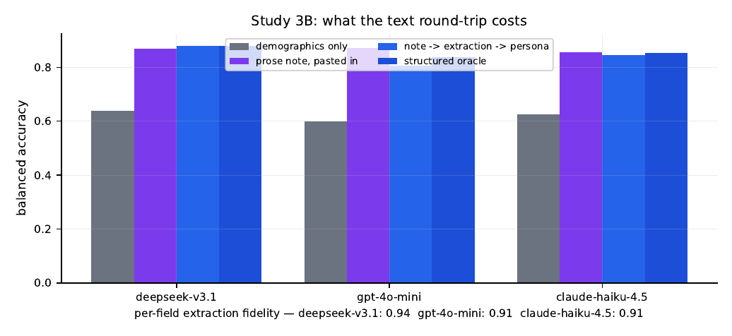
Read together with §4’s equivalence between simulating and asking, this closes a loop. Neither the persona framing nor the extraction schema buys accuracy over the plainest thing a user could do, which is to paste what they know about a person into a prompt. What the schema does buy is the ability to say which fields were used, where each came from, and what the model was told — the same provenance the placebo arm shows the model will not enforce for itself. That is a real product property, and it is an auditing property, not an accuracy one. A vendor claiming otherwise is claiming something these measurements do not support.
Study 4: the depth curve
Cells, and how deep a survey lets you go
A cell is an audience specification: demographic attributes fixed, everything else free. The prior study scored 74 cells at depths 1 and 2. Here the same six fields (sex, race/ethnicity, age band, education, income band, region) are crossed to depth 5, with one inclusion rule applied identically at every depth: at least 25 respondents and at least 25 units of weighted mass.
The share of crossings that clear that rule is itself a result, and it is what limits the study:
| depth | 1 | 2 | 3 | 4 | 5 |
|---|---|---|---|---|---|
| crossings observed | 27 | 296 | 1,665 | 4,549 | 4,990 |
| qualifying | 27 | 262 | 843 | 779 | 175 |
| share | 100.0% | 88.5% | 50.6% | 17.1% | 3.5% |
At depth 6 nothing qualifies at all. The survey, not the budget, sets the horizon.
Twenty cells are taken at each depth, selected at evenly spaced mass ranks rather than by taking the largest. Taking the largest is the obvious rule and it is the wrong one: it makes depth nearly collinear with cell mass, so a depth effect could never be separated from a thin-cell effect. Under mass-stratified selection, depth-1 cells span to and depth-4 cells span to , leaving enough overlap to control for mass explicitly.
The truth degrades too
Every comparison at depth is bounded by how well the survey itself resolves the cell. We estimate that per cell two ways: a stratified bootstrap over the ANES variance design (resampling primary sampling units within variance strata and recomputing the conditional), and a split-half reference. The two disagree in exactly the place it matters — split-half runs about twice the bootstrap in thin cells, because PSU resampling under-disperses when a cell spans few units — so the larger is used as the floor, and both are reported. No arm comparison appears in this paper without its floor drawn beneath it.
Arms
Every arm is one the prior study ended with, so depth-1 and depth-2 points act as a positive control against published numbers. Free arms: F, 200 fusion draws with the party read directly; M1, a weighted empirical conditional on 750,022 pooled CES and GSS rows with hierarchical backoff; M0, the training marginal. Paid arms on two models: A, 50 product-path personas elicited in character; V, verbalized sampling (Zhang et al. 2025) at 20 calls of five candidates; D and D7, direct readout of the vote distribution and of the full seven-point party distribution; and L, calibrated-label injection, run at depths 3–5 only, where the injected label is itself an extrapolation.
Arm B — naive repeated prompting of one backstory — is deliberately not re-run. The prior study established it as three times the error of every expert arm with collapsed dispersion, and four depths of confirmation would buy nothing. Its absence is recorded in the run summary rather than left to be noticed.
Two instrument choices follow corrections this program has already paid for. Every arm, including the free ones, is read through the same -draw sampling instrument: scoring an exact distribution against a sampled arm flatters the exact side, and this paper’s entire argument is a comparison between exactly those two kinds of arm. And the lookup baseline was found, during the free stage, to be matching cell criteria against a different education and income vocabulary than its own training rows use, so it had been silently backing off on two of six axes. Repaired here, the effect on the prior study’s 74 shallow cells is nil (mean 0.1174 to 0.1173) and on this study’s deep cells decisive (cells with no exact support at depth 3: 90% to 10%). A defect that changes nothing in one regime and everything in the next is an argument for re-auditing baselines when the regime moves, not only when the code does.
What the free stage already settles
Three of this study’s premises turned out to be wrong, and all three were wrong before a single paid call — which is the argument for running the free arms first.
The lookup does not collapse; it wins.
We expected the training-data lookup to degrade fastest, since it must back off where the generator interpolates. It does the opposite. Across depths 1 to 5 the lookup runs 0.099, 0.111, 0.144, 0.161, 0.145 while the fusion generator runs 0.116, 0.178, 0.178, 0.212, 0.201 — the lookup is better at every depth and degrades more slowly. Worse for the generator, the training marginal — one distribution, the same for every cell — runs 0.122, 0.183, 0.179, 0.214, 0.238, which is to say the generator barely separates from a constant at depths 2 through 4. Whatever the generative joint model is contributing in the deep regime, it is not distributional accuracy.
There is no unsurveyed stratum to find by crossing demographics.
The inclusion floor needs 25 of 6,222 ANES respondents, roughly 0.4% of the population. A 0.4% cell has on the order of 3,000 expected rows in a 750,022-row training corpus, so the reference survey runs out of resolution more than a hundred times sooner than the training data runs out of rows. The regime this study was built to reach is not reachable by crossing coarse demographics at all. It is reachable when a variable is missing rather than when a cell is thin: income is null for 92% of training rows, and the lookup’s backoff rate is driven almost entirely by whether the cell fixes income. That is a finding about where the support gap actually lives, and it relocates the product claim it was meant to test.
A missing variable and a thin cell are different failures, and we can now show it.
The argument above — that the support gap is variable-shaped rather than cell-shaped — was inferential in the first draft, resting on income being 92% null in the training population. It is testable, because we can create the two failures on purpose. Masking a variable the training data does have raises the lookup’s error on the cells that fix it: education 0.134 to 0.165, region 0.151 to 0.195, age band 0.148 to 0.173, with backoff going from zero fields to one in every case. Thinning the training population instead — keeping every variable but discarding rows until 750,022 becomes 22,350, a 33-fold reduction — costs 0.135 to 0.161 overall and changes the backoff structure not at all.
So a 33-fold thinning of the corpus costs about what masking a single variable costs, and only the masking changes what the estimator can condition on. The two failures are separable and they are not the same size.
The natural case sharpens it further, and complicates the story in a way worth stating. Cells that fix income have 100% zero exact support and back off a full field at every depth — and their error is not systematically worse (0.102–0.152 against 0.107–0.249 for cells that do not fix income). A missing variable costs you in proportion to what that variable would have told you, and income tells you comparatively little about party. The support gap is real, it is variable-shaped, and it is only a business opportunity when the absent variable is one that carries signal. That is a narrower claim than “audiences nobody surveyed” and it is the one the measurements support.
The gate fires, and it removes depth 1.
Comparing the aggregate free-arm difference at each depth to its own bootstrap uncertainty, depth 1 fails ($|{\rm F}-{\rm M1}| = 0.017$ against a half-width of 0.018) and depths 2 through 5 pass. Depth 1 is nevertheless retained in the paid stage, for a stated reason: it is the positive control against the prior study’s published numbers, not a place where this study expects to learn anything.
Results
24,400 calls, no failures. Table 3 and Figure 3 give bias-corrected total-variation distance by depth for every arm, with the survey’s own sampling error drawn beneath.
Asking has the steepest depth slope — and still the lowest error everywhere the survey can check.
The direct arm’s depth slope is the largest of any arm ( and total-variation per additional fixed attribute, both marginal intervals excluding zero). How far that ordering can be pushed depends on testing differences rather than comparing verdicts, so every arm-to-arm comparison below is a paired bootstrap in which both arms are refit on the same resampled cells. Paired, the direct arm’s slope exceeds verbalized sampling’s on both models ( and ) but is not distinguishable from the grounded arm’s ( , ) or from either free arm’s. So “asking degrades fastest” is a statement about point estimates and about one paired contrast, not a resolved ordering over all arms, and we state it that way.
What the direct arm does not do is lose its lead. It is still the
most accurate arm at depth 5 (0.125 and 0.153, against 0.171 and 0.214
for grounded personas). The margin narrows on deepseek-v3.1
—
to
,
with the depth-4 and depth-5 intervals now including zero — but does not
close, and on gpt-4o-mini it does not narrow at all.
H19 is partially supported on one model and unsupported on the
other.
Most of the generator’s apparent degradation belongs to the reference, not to the generator.
This is the result we did not anticipate, and it needs a paired test
to state honestly. Raw depth slopes for the fusion generator and the
training lookup are
and
,
both marginal intervals excluding zero; controlling for log cell mass
they fall to
and
.
An interval containing zero is not evidence of no effect — and here it
also contains the raw estimate — so the quantity that matters is the
reduction, resampled on the same cells. For the fusion
generator that reduction is
and resolves: the control removes most of its apparent depth slope. For
the lookup it is
and does not. For the direct arm it is
and
,
neither resolving — its slope is not reduced by the control. And for the
grounded arm on gpt-4o-mini the control moves the slope the
other way,
,
which is the strongest evidence that this control is doing something
other than costing precision.
Read together: what looked like a generative model failing on deep cells is, for the generator, mostly a survey failing on small ones; the direct arm shows no such reassignment. Depth and log cell mass correlate at over the 100 cells even under mass-stratified selection, so the control is fighting real collinearity and its standard errors are inflated accordingly — but a depth comparison that omits it is measuring the survey. The control is a linear term in log cell mass in an ordinary least-squares fit with cells as the resampling unit; replacing it with a quadratic in log mass moves no coefficient by more than 0.002 and changes no interval’s relationship to zero (Appendix 13).
Prompting for a spread has the shallowest slope.
Verbalized sampling has the smallest depth slope of the three paid
arms
(
and
),
and under the mass control it is flat or negative on both models.
Paired, it is shallower than the direct arm on both
(,
,
both resolving) and shallower than the grounded arm on
gpt-4o-mini
(
)
though not on deepseek-v3.1. At depth 5 on
deepseek-v3.1 it also overtakes grounded personas on level
(0.131 against 0.171). The most robust simulation-shaped arm we measured
in the deep regime is a prompt.
The support indicator does not work, and should not ship.
Pooled across all cells, the fusion arm’s error correlates with the training mass behind the cell, which clears the preregistered gate. Within depth it collapses: , , , , at depths 1 through 5, failing the gate at three of five and changing sign twice. The pooled correlation is depth in disguise. H21 is falsified, and its preregistered kill switch fires: a confidence indicator built from this quantity would not indicate confidence, and the roadmap item that depended on it does not survive.
The same ordering holds on the harder target, and one grounded property survives.
On the full seven-point party distribution the gap is wider, not
narrower: direct readout runs 0.137 to 0.248 across depths on
deepseek-v3.1 and 0.164 to 0.302 on
gpt-4o-mini, against 0.304 to 0.402 and 0.339 to 0.419 for
grounded personas. Nothing about the deep regime rescues simulation on
the finer-grained outcome either.
One thing does survive, and it is the property the prior study identified as the grounded arm’s genuine contribution. Within-cell dispersion, the ratio of predicted to true standard deviation, stays inside the preregistered band at every depth on both models (0.81–0.91 and 0.91–1.04), and verbalized sampling stays inside it too (0.76–0.90). Grounded personas keep producing honestly-spread populations as the specification deepens, even as their level accuracy falls behind. That is worth stating precisely because it is the narrow claim the measurements do support: not that the room is right, but that it is not collapsed.
The survey can still adjudicate everywhere we looked.
Median arm-to-arm spread exceeds the sampling floor at every depth (0.118 against 0.014 at depth 1, 0.127 against 0.045 at depth 5), so H22 reports no resolution failure within the range this instrument reaches. The floor triples across that range while the spread stays flat, though, and the trend is what matters: the margin of decidability is shrinking, and a split-half estimator — biased upward by about a factor of two, since it is taken over two independent halves, and therefore reported only as a diagnostic — already runs 0.040 to 0.078 over the same depths. One or two levels further down and these comparisons stop being decidable on this survey.
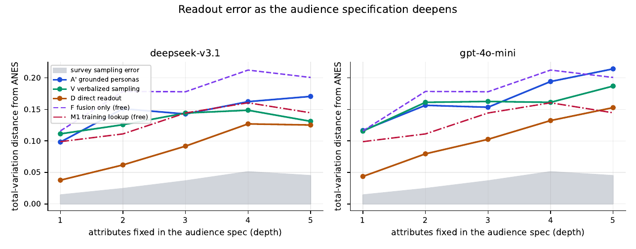
| Arm | |||||
|---|---|---|---|---|---|
| F fusion only (free) | 0.116 | 0.178 | 0.178 | 0.212 | 0.201 |
| M1 training lookup (free) | 0.099 | 0.111 | 0.144 | 0.161 | 0.145 |
| M0 training marginal (free) | 0.122 | 0.183 | 0.179 | 0.214 | 0.238 |
| deepseek-v3.1 | |||||
| A’ grounded personas | 0.098 | 0.151 | 0.143 | 0.162 | 0.171 |
| V verbalized sampling | 0.111 | 0.126 | 0.144 | 0.149 | 0.131 |
| D direct readout | 0.038 | 0.062 | 0.092 | 0.127 | 0.125 |
| gpt-4o-mini | |||||
| A’ grounded personas | 0.117 | 0.157 | 0.153 | 0.194 | 0.214 |
| V verbalized sampling | 0.116 | 0.161 | 0.163 | 0.161 | 0.187 |
| D direct readout | 0.044 | 0.080 | 0.102 | 0.132 | 0.153 |
| survey sampling error | 0.014 | 0.025 | 0.037 | 0.051 | 0.045 |
What this means for simulation products
The inversion is real, and it is not a licence for the product claim it was supposed to justify.
The prior study’s negative result was about invented people, and Study 3 confirms it stops exactly where the theory said it would: measured attributes move individual-level accuracy by about a quarter of the scale, sampled ones move it backwards, same pipeline and same respondents. A vendor may therefore say, with evidence, that knowing real things about a person changes what a simulation of them is worth. What that vendor may not say is that the simulation is doing the work. On the same measurements, asking the model about the person is as accurate as embodying them, the two agree on 92–96% of individuals, pasting the source material into a prompt is as good as the structured pipeline, and a logistic regression on the same attributes pulls ahead as the attribute count grows.
Compliance is the mechanism, and it is a safety property before it is a performance one.
The models follow a disclosed attribute more tightly than that attribute predicts the outcome, and follow a demographically matched stranger’s attribute nearly as tightly. Anything that reaches the persona will be obeyed roughly in proportion to how confidently it is stated, whether or not it is true of the subject. A system that assembles personas from real material inherits that property directly: an extraction error, a stale fact, or a mismatched record does not degrade gracefully, it gets acted on. The placebo arm is the cheapest possible test of whether a deployment has this problem, and we would argue any product making individual-level claims should run it and publish the number.
Structure buys provenance, not accuracy, and that is still worth something.
Study 3B is the clearest statement of the trade. Extracting prose into a schema and rebuilding the persona costs nothing measurable, so the pipeline is not destroying information — but it does not beat pasting the prose in either. What it adds is the ability to say which fields were used, where each came from, and what the model was shown. Given that the same experiments show the model will not police provenance itself, an auditable field-level trail is the feature, and it should be sold as one rather than dressed up as an accuracy gain.
Both studies point the same way: the defensible asset is the audit, not the readout.
This is now the third result in this program with that shape. Population readouts on well-surveyed cells were commodity; steering was bounded by two channels that can be measured in advance without a model; and individual-level accuracy turns out to be available to anyone who can write the facts into a prompt. In each case the thing that is not commodity is knowing — and being able to demonstrate — how far the answer can be trusted: which surveys calibrated it, how much support stands behind the cell, whether the attributes belong to the person they claim to, and how much of the ground truth is itself noise.
The deep-cross market does not exist in the form it was imagined.
Study 4 was commissioned to gate a product feature: audiences nobody has surveyed, where a generative joint model would be the only arm that can answer. The measurement says the premise is wrong twice over. Crossing coarse demographics does not reach an unsupported cell, because the reference survey runs out of resolution more than a hundred times before a 750,000-row training corpus runs out of rows; and where the specification does deepen, asking the model remains the most accurate arm, with prompting for a spread the most robust one. The support gap is real but it lives on a different axis — a variable nobody collected, not a cell nobody reached — and that is a different feature with a different validation.
Publish the floor, not just the number.
Every comparison in Study 4 sits above the survey’s own sampling error, and that error doubles from depth 1 to depth 5. One more level and the arms stop being distinguishable on this instrument at all. We think this generalises past our setting: any benchmark that scores synthetic populations against a survey is eventually measuring the survey, and papers in this area should be reporting where that boundary falls rather than reporting differences on the far side of it. Estimating it is cheap — a stratified resample of the reference survey’s own design — and it changed our reading of two hypotheses.
A confidence indicator has to be tested within the regime it will be used in.
Pooled across cells, the generator’s training support predicts its error well enough to look shippable. Within depth — which is how a user would actually encounter it, comparing two equally deep specifications — it predicts nothing, and changes sign. Had we tested only the pooled correlation we would have shipped a number that tracked depth while appearing to track confidence.
Limitations
Survey answers are not journalism. Study 3’s disclosures are coded responses to well-posed questions, delivered in a fixed register. Real material about a real person is partial, contradictory, undated, and mixed with irrelevance. Study 3B moves one step toward that by delivering the same facts as prose and recovering them, but a template-generated note is still far tidier than a news profile or an interview transcript, and the extraction fidelity we measure is an upper bound on what a messier corpus would give. We do not claim to have run a corpus study, and the gap is the obvious next experiment.
One outcome domain, with one probe outside it. Both studies’ headline results score U.S. vote and party identification, which are unusually well predicted by attitudes and unusually well represented in pretraining. Study 3C moves one step out, to the weakest-signal item in the same pool, and finds the disclosure effect essentially gone — which bounds the headline usefully but is still the same survey, the same respondents and the same broadly political domain. A disclosure curve for consumer preference, health behaviour or workplace judgement could differ again, and nothing here says where between those two points such an outcome would fall.
The deep regime is bounded by the survey, not by the method. Study 4 stops at depth 5 because ANES has no qualifying cells at depth 6, and the depth-5 cells it does have are thin enough that the truth floor is a first-order term rather than a footnote. Claims about still-deeper specifications — which is where the commercial interest actually lies — are outside what this instrument can adjudicate, and we mark where that boundary falls rather than extrapolating past it.
Depth and mass cannot be fully separated. Mass-stratified selection reduces their correlation and leaves enough overlap for an explicit control, but deep cells are smaller cells in the population as well as in the sample, and no selection rule inside one survey can break that entirely. Every depth slope is therefore reported twice, raw and mass-controlled, and we treat a slope that does not survive the control as a thin-cell effect.
Two models in Study 4, three in Study 3. The prior study’s seven-model panel established that whether grounding helps is predicted by baseline calibration; Study 3 spans that range deliberately but is not a census of models, and Study 4 keeps the prior study’s two for continuity. Backend nondeterminism and undisclosed model updates apply here as everywhere.
The compliance diagnostic has alternatives we have not exhausted. We measure obedience with one item, in one polarity, in one position in the prompt. Presentation artefacts — item order, label semantics, the direction the scale runs — are plausible partial explanations and we have not ruled them out with paraphrase or randomisation experiments. What makes us confident the effect is not purely presentational is the placebo: the same prompt structure with a stranger’s value produces nearly the same grip, which no presentation account explains on its own.
The variable-versus-cell demonstration is an ablation, not a field test. Masking a variable we have and thinning a corpus we have shows the two failures are separable and differently sized. It does not show what happens when a variable was never collected by anyone, which is the case the product claim is actually about, and which no ablation on an existing corpus can reach.
The placebo’s donors are close matches. Donors matched on a mean of 5.61 of six demographic fields, which is the point — a plausible stranger, not a random one — but it also means the placebo is a conservative test of false specificity. A random donor would presumably hurt more, and would tell us less.
Ethics
Study 3 is a study of how well a language model can infer a real person’s political behaviour from facts about them, which is also a description of a profiling capability. We think the honest position is that the capability exists whether or not it is measured, and that measuring it is what makes its limits arguable. Three properties of the design bear on the risk directly.
The respondents are pseudonymous participants in a public probability survey, identified only by row position in a file that thousands of researchers already hold. No attribute in the pool identifies a person, and no persona is retained.
The placebo arm is the ethically load-bearing one. If a persona built from a demographically matched stranger’s answers predicts as well as one built from the subject’s own, then a system claiming to represent a specific person is really representing their demographic neighbourhood while presenting the output as individual. Reporting that arm alongside the accuracy number is what keeps a provenance claim falsifiable, and we would argue any deployed system making individual-level claims owes its users the same comparison.
Study 4’s risk runs the other way. A generative model answers a question about a five-way demographic crossing with the same fluency as a question about one attribute, and nothing in its output signals which of the two it has grounds for. The prior study argued that a steering claim without its audit is marketing; the same applies to a deep-cell readout. If the support statistic tested in §5 predicts error, a system can ship it and let users discount accordingly; if it does not, the honest response is to say so rather than to ship a confidence indicator that does not indicate confidence. We report which of those two we found.
Finally, both studies concern U.S. electoral behaviour, a domain where synthetic-population claims have obvious potential for misuse in targeting and persuasion. Nothing here improves persuasion; the results bound what these systems can and cannot know, which is if anything a deflationary contribution.
Availability
The system under study is commercial software; code and model artifacts are not public, and are available to partners and clients under agreement. The evaluation protocol is fully public: both studies run against a public probability survey (ANES 2020) through public LLM APIs, and the appendices specify the item pool with codebook variable ids, the cell enumeration rule, every prompt template, and the calibration and bootstrap procedures in enough detail to reimplement. A hosted evaluation endpoint for third-party audit reproduction is under exploration.
Preregistration and amendments
Both studies’ hypotheses, arms, splits or cells, metrics, decision rules and budget ceilings were written down before any paid call. The full preregistrations and lab notebooks are maintained with the code.
Adversarial review.
Before the confirmatory runs, both preregistrations were put through a structured adversarial critique: four independent lenses (survey statistics, confounding, reviewer-perspective, implementability), each objection then independently verified against the repository with instructions to refute by default. Thirty-two objections were raised and twenty-six survived. Six were blocking, and all six were fixed before spending. We report them because a defect found before spending is the cheapest kind, and because two of them are the sort that produce publishable-looking numbers.
A coverage rule voided its own robustness check. “Haven’t thought much about this” was treated as missing data. It is not missing — it is a disclosable fact about a person, given by 10–14% of voters — and treating it as missing pushed all five ANES seven-point scales below the 90% coverage floor. That removed ideology from the pool, which made the study’s “without ideology” robustness check byte-identical to the result it was checking. Recoded as a named level at the scale midpoint: coverage for ideology moves from 0.864 to 0.999, all 22 items qualify, and the harness now refuses to run if that check would be vacuous.
The evaluation split was weighted twice. It is drawn with probability proportional to survey weight, and was then weighted again at scoring, i.e. by . Corrected; the demographics-only baseline moves from 0.697 to 0.640.
A gate was hardcoded to pass. Study 4’s Stage-0 gate was the literal
gate = True, printed with a comparison beside it that never fed the decision. Replaced by a per-depth test of the aggregate free-arm difference against its own bootstrap uncertainty — which then removed depth 1, retained on stated grounds as a positive control.A vocabulary reconciliation was wrong. A map between training-data and cell income bands, added the same day, identified two different scales (one corpus has no income at all; the other’s bands are constant-dollar), converting a visible backoff into an invisible mis-conditioning that made the baseline worse while making it look better supported. Removed; the education map, a genuine naming difference for the same construct, stays.
The noise-floor bootstrap froze the thinnest cells. Strata holding a single primary sampling unit were copied verbatim into every draw, freezing 74% of a cell’s members at depth 4 — precisely where the study’s claims live. Singletons are now pooled and resampled; the depth-4 floor rises from 0.036 to 0.046.
Sampling bias was uncorrected and arm-dependent. Reading a distribution from draws inflates total-variation distance by an amount depending on both and how far the arm is from the truth, so it differs across arms at equal . Now estimated per arm per cell against the actual truth, with raw and corrected values both reported.
Two further changes followed from the critique without being defects: arm L (calibrated-label injection) was cut because it appears in no hypothesis, funding a second repeat of the grounded arm; and the weak-attribute pool was promoted to Study 3’s primary curve, because the full pool’s most predictive item is the 2020 Republican candidate’s signature policy and its supervised curve is a step rather than a dose-response.
Declined, with reasons.
A nested-ladder redesign for Study 4 (select deep anchors, generate their ancestors, estimate paired within-chain contrasts) is the strongest proposal the critique produced and is right about the composition confound — every deep race-fixing cell in our set is white. It was declined because it rebuilds the cell structure after the free stage had run, and adopted in part instead: depth slopes are reported raw and mass-controlled, and the absence of qualifying non-white deep cells is reported as a finding about survey resolution. A prior-odds threshold for the direct arm was declined because it would give that arm a fitted degree of freedom the in-character arm does not have.
A retained pre-amendment run.
Study 3’s first confirmatory run (15,600 calls, the 16-item no-ideology pool, scoring) completed before the amendments and is retained as a labelled sensitivity run rather than discarded. Its pattern is the one the corrected design then re-measured. Study 4’s first run was stopped at 39% and discarded, because its design had changed materially and finishing it would have spent roughly $1.90 on data the paper could not use.
The measured-attribute pool
All twenty-two candidates were verified against
anes_timeseries_2020_userguidecodebook_20220210.pdf —
variable id, question wording, and every value label — before use.
“Rank” is the position in the fit-split predictive ranking;
bold marks the sixteen items the disclosure curve uses.
All twenty-two clear the 90% coverage floor. Coverage is the
survey-weighted share of the 6,222 ANES 2020 voters giving
a substantive answer, where “Refused”, “Don’t know”, “Other (specify)”
and inapplicable-by-universe count as missing. “Haven’t thought much
about this”, offered only by the five seven-point scales and taken by
10–14% of voters, does not: it is a fact about the person,
scored as a named level at the scale midpoint. Treating it as missing
dropped all five scales below the floor and voided a robustness check
(Appendix 10, item 1).
| Rank | Variable | Item | Levels | Coverage |
|---|---|---|---|---|
| 1 | V201424 | Favor Or Oppose Building A Wall On Border With Mexico | 3 | 0.999 |
| 2 | V201200 | 7Pt Scale Liberal-Conservative Self-Placement | 8 | 0.999 |
| 3 | V201262 | 7Pt Scale Environment-Business Tradeoff: Self-Placement | 8 | 0.999 |
| 4 | V201306 | Federal Budget Spending: Tightening Border Security | 3 | 0.997 |
| 5 | V201321 | Federal Budget Spending: Protecting The Environment | 3 | 0.999 |
| 6 | V201255 | 7Pt Scale Guaranteed Job-Income Scale: Self-Placement | 8 | 0.998 |
| 7 | V201336 | Std Abortion: Self-Placement | 4 | 0.964 |
| 8 | V201246 | 7Pt Scale Spending & Services: Self-Placement | 8 | 0.998 |
| 9 | V201312 | Federal Budget Spending: Welfare Programs | 3 | 0.996 |
| 10 | V201318 | Federal Budget Spending: Aid To The Poor | 3 | 0.999 |
| 11 | V201249 | 7Pt Scale Defense Spending: Self-Placement | 8 | 0.998 |
| 12 | V201417 | Us Government Policy Toward Unauthorized Immigrants | 4 | 0.994 |
| 13 | V201303 | Federal Budget Spending: Public Schools | 3 | 0.999 |
| 14 | V201416 | R Position On Gay Marriage | 3 | 0.993 |
| 15 | V201309 | Federal Budget Spending: Dealing With Crime | 3 | 0.996 |
| 16 | V201433 | Is Religion Important Part Of R Life [Revised] | 5 | 0.999 |
| 17 | V201415 | Should Gay And Lesbian Couples Be Allowed To Adopt | 2 | 0.988 |
| 18 | V201453 | Attend Religious Services How Often | 5 | 0.995 |
| 19 | V201412 | Does R Favor/Oppose Laws Protect Gays/Lesbians Against Job Discrimination | 2 | 0.994 |
| 20 | V201300 | Federal Budget Spending: Social Security | 3 | 0.997 |
| 21 | V201233 | How Often Trust Government In Washington To Do What Is Right [Revised] | 5 | 0.997 |
| 22 | V201006 | How Interested In Following Campaigns | 3 | 1.000 |
With ideology restored to the pool, the sampled-versus-measured contrast is available at the field level as well as the arm level: arms P1 and P1-flat state a sampled ideology where P2() states the respondent’s measured one, in the same sentence frame.
Two items are coded on an axis that is not their ANES code order, and both recodings are declared in the frozen item table rather than applied at analysis time: the federal-spending battery (“increased” 1, “kept the same” 3, “decreased” 2 becomes on an increase-to-decrease axis) and the border-wall item (“favor”, “neither”, “oppose”).
Prompts
The elicitor is unchanged from Grey (2026): a system message instructing the model to role-play a specific American voter answering a short survey in November 2020 and to reply with a single JSON object, followed by the persona text and two items — 2020 presidential vote (“biden”, “trump”, “other”) and seven-point party identification. Parsing is tolerant of code fences and surrounding prose; unparseable completions are counted, not silently dropped.
Study 3, arm P2 (measured).
The shared demographic block, then one first-person sentence per disclosed attribute. For a respondent disclosing four attributes:
I am a white man in my late 30s/early 40s. I live in OH. I have a high school education. My household income is over $150,000. I favor building a wall on the border with Mexico. I think federal spending on tightening border security should be increased. I think federal spending on protecting the environment should be kept the same. I think federal spending on welfare programs should be decreased.
Study 3, arm P1-flat (sampled).
Identical format, with the fusion posterior’s decoded fields in place of the measured ones. The contrast between the two is exactly the contrast the study is about, and it is visible in what the generator has to offer:
I am a Black woman in my late 60s/early 70s. I live in OH. I have a high school education. My household income is under $35,000. Politically I’d describe myself as conservative. I go to religious services every week. I’m warm and cooperative. I’m organized and dependable. I’m outgoing and sociable.
Note what is absent: not one of the issue positions that carry the
individual-level signal appears, because the generator’s
issue_stances field decodes empty. The sampled arm is not a
weaker version of the measured arm; it is a different set of fields.
Study 3, arm P4 (direct).
The same facts in the third person, asked as a probability at temperature 0:
Here is what is known about one real American voter in November 2020.
A Black woman aged 65-74, with a high school education, a household income under $35,000, living in the midwest. This person neither favors nor opposes a border wall; wants federal spending on tightening border security kept the same; wants federal spending on protecting the environment increased; wants federal spending on welfare programs increased.
Estimate: (1) the probability this person voted for Trump rather than Biden; (2) their 7-point party identification (1=Strong Democrat, 4=Independent, 7=Strong Republican).
Return exactly: {"trump_prob": 0.xx, "party7": N}
Study 3B, the profile note.
Generated from a template with lexical variation and no language model, so the note carries the disclosed facts and nothing else:
What we know about a white man aged 35-44, with a high school education, a household income over $150,000, living in the midwest: The file notes that this person wants federal spending on public schools increased. Our notes say this person believes abortion should be permitted only for rape, incest, or danger to the woman’s life. […] In interviews this person favors building a border wall with Mexico.
The extraction call presents the note and the frozen schema with the permitted labels per field and an explicit null option, at temperature 0.
Study 4.
Arm
A
uses the shipped ProfileData.to_first_person_intro()
rendering with the leakage mask of Grey (2026): the political-stance line is
rebuilt as ideology only, since the shipped string embeds party
identification and turnout. Arm L is the cell backstory plus one sampled
ideology sentence. Arms D, D7 and V reuse that paper’s prompts verbatim
so the shallow-depth points reproduce published numbers.
Cell enumeration and the truth noise floor
Enumeration.
All -way crossings of six demographic fields over 6,222 ANES 2020 voters, with one inclusion rule at every depth: at least 25 respondents and at least 25 units of weighted mass.
| depth | 1 | 2 | 3 | 4 | 5 |
|---|---|---|---|---|---|
| crossings observed | 27 | 296 | 1,665 | 4,549 | 4,990 |
| qualifying | 27 | 262 | 843 | 779 | 175 |
| share | 100.0% | 88.5% | 50.6% | 17.1% | 3.5% |
At depth 6, zero of 1,717 observed crossings qualify.
Selection.
Twenty cells per depth at evenly spaced mass ranks, capped at four per field-combination. Taking the largest cells instead would make depth nearly collinear with mass and the depth effect unidentifiable; under this rule depth-1 cells span to and depth-4 cells to , leaving enough overlap for the explicit mass control that §5 relies on.
The floor.
Per cell, a stratified bootstrap over the ANES variance design (400 draws, resampling primary sampling units within variance strata, weights applied inside each draw), plus a split-half reference. Strata with a single sampling unit are pooled into one pseudo-stratum per cell and resampled rather than copied; at depth 4 that affects a median 74% of members. Split-half over two independent halves is a biased estimator of the full-sample error — each half carries about times it — so it is halved and reported as a diagnostic, and no decision rule uses it.
Mass control and its sensitivity.
Depth slopes are ordinary least squares of per-cell total-variation distance on depth, with cells as the bootstrap resampling unit (4,000 draws) and no weighting: cells are the units of analysis, not respondents. The control adds as a second regressor. Replacing it with gives: fusion against linear; lookup against ; direct readout and against and ; grounded personas and against and . No coefficient moves by more than 0.002 and no interval changes its relationship to zero.
How the obedience statistic is computed.
For a given arm and model, over the eval respondents that arm scored:
the Pearson correlation between the disclosed item’s monotone score (the
frozen item table’s numeric, not the raw ANES code) and an
indicator for the arm predicting a Republican vote. Unweighted, because
the eval split is drawn with probability proportional to survey weight
and is therefore self-weighting. The top-ranked item is used throughout,
so every row of the obedience table is the same item on the same
respondents; only what the persona was told about it varies. The truth
reference is the same correlation with the respondents’ actual
vote in place of the prediction. In the placebo arm the score is the
donor’s, not the subject’s, since the question is whether the
model follows what it was told. The item’s score axis runs
favour-to-oppose, which is why the correlations are negative; their
magnitude is what the argument turns on.
Sampling-bias correction.
For an arm reporting from draws against truth , we estimate over 600 redraws and report alongside the raw value. Estimating against the actual truth rather than a generic floor matters: the two differ by a factor of four at these arms’ accuracies. Free arms are read at , where the correction is negligible; the direct arms emit a distribution and carry none.
References
Part of the AnthroSim research program map.